class: center, middle, inverse, title-slide # Assumptions and Diagnostics --- ## Last time * (One-way) Analysis of Variance --- ## Today * Assumptions of GLM regression models * Diagnostics (checking those assumptions) --- ## BLUE Best Linear Unbiased Estimate of beta `\((\beta)\)` -- * Unbiased * Efficient * Consistent ??? Unbiased: what does it mean for an estimate to be biased? How did we describe the bias of variance? Efficient: smallest standard error (best) Consistent: as N increases, standard error decreases --- ## Assumptions of the regression model 1. No measurement error 2. Correctly specified form 3. No omitted variables 4. Homoscedasticity 5. Independence among the residuals 6. Normally distributed residuals --- ## What happens if we violate assumptions? 1. Biased regression coefficients 2. Biased standard errors --- ## 6 assumptions |Violated Regression Assumption | Coefficients | Standard Errors| |-------------------------------|--------------|-----------------| |1. Measured without error | Biased | Biased | |2. Correctly specified form | Biased | Biased | |3. Correctly specified model | Biased | Biased | |4. Homoscedasticity | | Biased | |5. Independent Errors | | Biased | |6. Normality of the Errors | | Biased | --- ## How do we detect violations? | Assumption | Detection | |-------------------------------|--------------------------------| |1. Measured without error | Reliability | |2. Correctly specified form | Residuals against predicted | |3. Correctly specified model | Theory, endogeneity test | |4. Homoscedasticity | Residuals against predicted | |5. Independent Errors | Research Design | |6. Normality of the Errors | q-q plot or distribution | --- ```r library(here) ``` ``` ## here() starts at /Users/sweston2/Google Drive/Work/Teaching/Courses/Graduate/Statistics and Methods Sequence/psy612 ``` ```r a_data <- read.csv(here("data/anxiety.csv")) library(broom) model.1 <- lm(Anxiety ~ Support, a_data) aug_1<- augment(model.1) aug_1 ``` ``` ## # A tibble: 118 x 9 ## Anxiety Support .fitted .se.fit .resid .hat .sigma .cooksd .std.resid ## <dbl> <dbl> <dbl> <dbl> <dbl> <dbl> <dbl> <dbl> <dbl> ## 1 10.2 6.16 8.68 0.245 1.51 0.0137 2.10 0.00366 0.725 ## 2 5.59 8.91 7.54 0.193 -1.95 0.00850 2.09 0.00376 -0.937 ## 3 6.58 10.5 6.86 0.220 -0.278 0.0111 2.10 0.000100 -0.134 ## 4 8.95 11.5 6.48 0.251 2.47 0.0144 2.09 0.0103 1.19 ## 5 7.60 5.55 8.93 0.269 -1.33 0.0165 2.10 0.00346 -0.642 ## 6 8.16 7.51 8.12 0.206 0.0368 0.00966 2.10 0.00000153 0.0177 ## 7 9.08 8.56 7.69 0.193 1.39 0.00850 2.10 0.00192 0.669 ## 8 3.41 4.1 9.53 0.334 -6.12 0.0255 2.02 0.115 -2.96 ## 9 8.66 5.39 9.00 0.276 -0.340 0.0173 2.10 0.000237 -0.164 ## 10 4.85 13.9 5.47 0.362 -0.620 0.0299 2.10 0.00139 -0.301 ## # … with 108 more rows ``` --- ## Residuals Residuals are your best diagnostic tool for assessing your regression model. Not only can they tell you if you've violated assumptions, but they can point to specific cases that contribute to the violations. This may help you to: * Notice patterns, which may lead you to change your theory * Remove problematic cases * Improve your research design --- 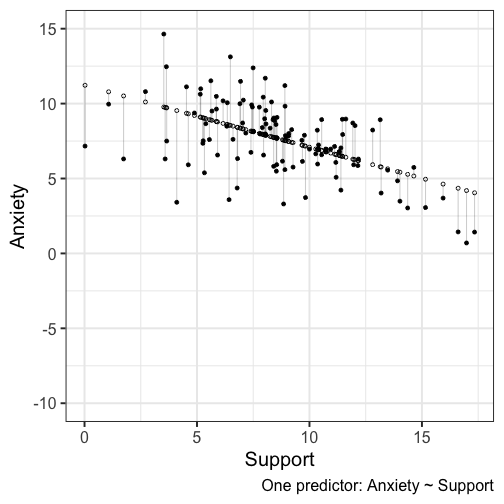<!-- --> --- 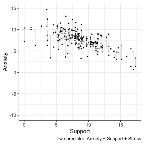<!-- --> We can add stress to the model to see how this changes --- ## 1) Measurement Error Assumption 1: No measurement error in our independent variables * How does measurement error affect our coefficient estimates? * How does measurement error affect our the standard errors of the coefficients? * How can we check this assumption? ??? If there is measurement error, our coefficient estimates will always UNDERestimate the true parameter. This is because `$$r_{XY} = \rho\sqrt{r_{XX}r_{YY}}$$` Measurement error inflates our standard errors, because they add error There is ALWAYS measurement error. What do we do about this? --- ## 2) Form Assumption 2: Correctly specified form 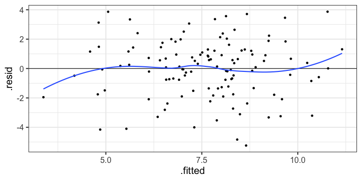<!-- --> ??? Underestimates `\(R^2\)` --- ## 3) Model Assumption 3: Correctly specified model - This is especially important for multiple regression. - Two problems: 1. "Over control" and your coefficient is no longer interpretable 2. "Under control" and your coefficient is no longer interpretable --- ## 3) Model ### Correctly specified model Cohen and Cohen (1983) discuss several problems associated with the inclusion of covariates/multiple independent predictors in a model. Those problems were: 1. Computational accuracy (not a problem now, because computers) 2. Sampling stability (tolerance) 3. Interpretation --- ## 3) Model ### Correctly specified model: Tolerance Recall that, computationally, including multiple predictors in your model requires adjusting for the overlap in these predictors. `$$\large se_{b} = \frac{s_{Y}}{s_{X}}\sqrt{\frac {1-R_{Y\hat{Y}}^2}{n-p-1}}\sqrt{\frac{1}{1-R_{12}^2}}$$` (in a two-predictor regression) Tolerance is: `$$\large 1-R_{12}^2$$` --- ## 3) Model ### Correctly specified model: Tolerance If your two independent predictors are highly correlated, tolerance gets smaller. * As tolerance gets smaller, the standard error gets larger. This is referred to as variance inflation. The **variance inflation factor** is an index to assess this problem. `$$\text{VIF} = \frac{1}{\text{Tolerance}} = \frac{1}{1-R^2_{12}}$$` * As the standard error becomes larger, the confidence intervals around coefficients becomes larger. When confidence intervals around estimates are large, then we say the partial coefficient estimates are *unstable.* --- ## 3) Model ### Tolerance VIF is not bounded, but generally large numbers (greater than 5 or 10, based on who's giving you the heuristic) indicates a problem. ```r library(car) vif(model.2) ``` ``` ## Support Stress ## 1.378785 1.378785 ``` The lesson from tolerance is that, as you add predictors to your model, it is best to select predictors that are not correlated with each other. What about (3) Interpretation? --- ## 3) Model ### Lynam et al (2006) -- Main takeaways: * Partialling changes the meaning and interpretation of a variable. * Partialling only takes variance away from the reliable `\((r_{XX})\)` part of a measurement. * Nothing is a good substitute for good theory and reliable measurement. * Always present zero-order correlations. ??? * It is difficult to know what construct an independent variable represents once the shared variance with other constructs has been removed * PARTIALLING CHANGES VARIABLES * Partialling only comes from the reliable part of the measurement -- if a scale has reliability .7 and correlates with another variable at .3, the partialling out the covariate removes .3 of the valid .7 variance or 9% out of 49% * Heterogeneous measures run the risk of greater dissimilarity following partialling. Empirical work: ~ 700 male inmates completed PCL-R assess psychopathy (interview coding) APSD (self-report) PRAQ proactive and reactive aggression EPQ PPI also psychopathy - partialling out sub-scales -- some correlations are even negative Good statistics cannot overcome poor measurement and bad theory - always present --- ## 3) Model ### Endogeniety Back to correctly specified models. 2. "Under control" and your coefficient is no longer interpretable **Endogeniety** is when your your error term is associated with a predictor. - Typically when you leave out an important predictor. - Can also occur if you "condition on a collider". Many ways this can happen but one common one is selecting a sample (clinical students, college students) that is associated with your variables of interest (e.g., emotion regulation, memory ability) ??? Underestimates `\(R^2\)` --- ## 3) Model ### Endogeniety ```r ggplot(aug_1, aes(x = Support, y = .resid)) + geom_point() + geom_smooth() + labs(caption = "One predictor: Anxiety ~ Support") + theme_bw(base_size = 20) ``` <!-- --> --- ## 4) Homoscedasticity **Homoscedasticity** is the general form of "homogeneity of variance." .pull-left[ **homogeneity of variance** * the variance of an outcome is the same across two (or more) groups * Levene's test ] .pull-left[ **Homoscedasticity** * the variance of an outcome is the same across all levels of all continuous predictor variables * visual inspection of residuals by fitted values ] --- ## 4) Homoscedasticity 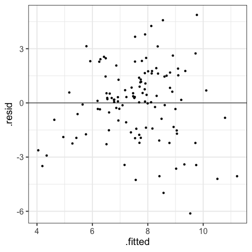<!-- --> --- ## 4) Homoscedasticity .pull-left[ 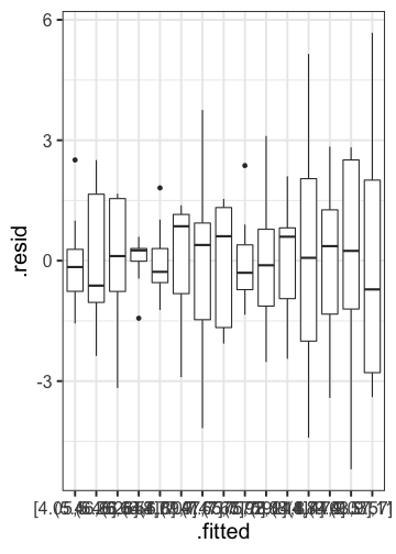<!-- --> ] .pull-right[ ```r aug_1 %>% mutate(.fitted = cut_number(.fitted, 15)) %>% group_by(.fitted) %>% mutate(.resid = .resid - mean(.resid)) %>% ggplot(aes(x=.fitted, y=.resid)) + geom_boxplot() + theme_bw(base_size = 20) ``` ] --- ## 5) Independence among the errors .pull-left[ 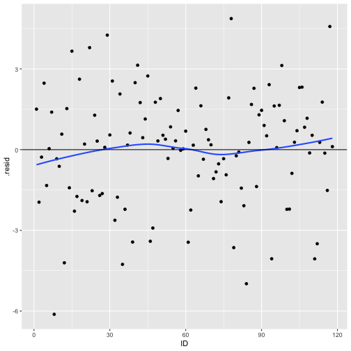<!-- --> ] .pull-right[ ```r aug_1$ID <- c(1:118) ggplot(data = aug_1, aes(x=ID, y = .resid)) + geom_point() + geom_smooth(se = F) + geom_hline(yintercept = 0) ``` ] --- ## 6) Normality of the errors ```r ggplot(data = aug_1, aes(x= .resid)) + geom_density(fill = "purple") + xlim(-10, 10) + theme_bw(base_size = 20) ``` 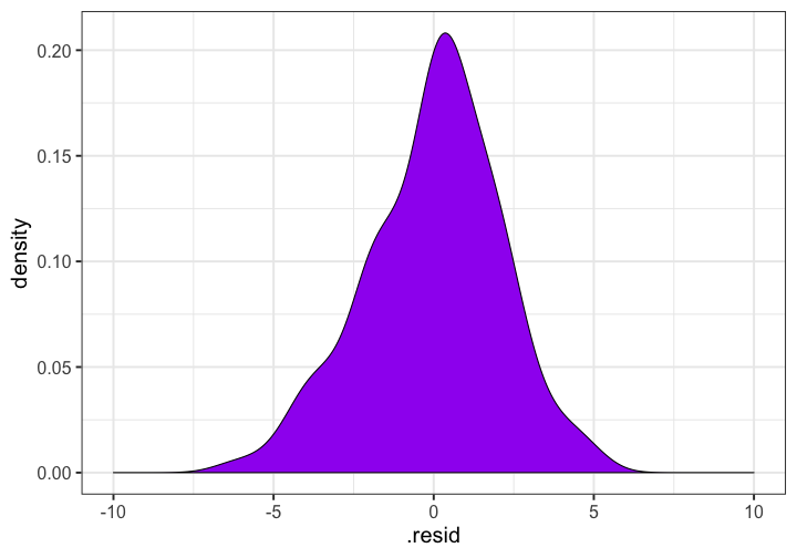<!-- --> --- ## 6) Normality of the errors ```r ggplot(model.1) + stat_qq(aes(sample = .stdresid)) + geom_abline() + theme_bw(base_size = 20) ``` 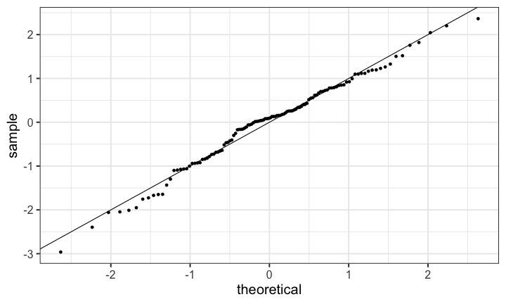<!-- --> --- ## 6) Normality of the errors ```r library(car) qqPlot(model.1) ``` 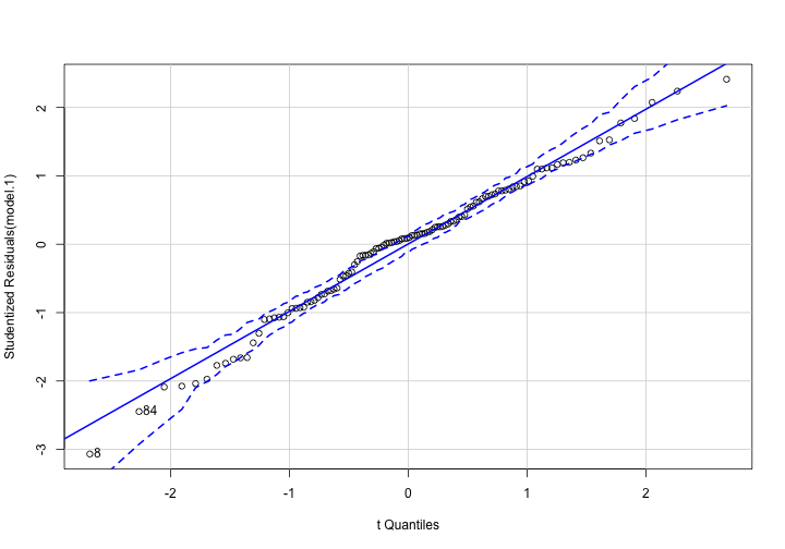<!-- --> ``` ## [1] 8 84 ``` ```r #base plot function too #plot(model.1, which = 2) ``` --- ## Violations of assumptions How can we address violations of assumptions of regression? | Assumption | Fix | |-------------------------------|----------------------------------| |1. Measured without error | SEM, factor scores, more data, better design | |2. Correctly specified form | Different model | |3. Correctly specified model | ¯`\_`(ツ)`_`/¯ & specificity analyses| |4. Homoscedasticity | Bootstraps, WLS, transformations | |5. Independent Errors | Use different analysis method | |6. Normality of the Errors | Additional IVs, different form | --- ## Violations of assumptions ### Robustness Regression models are considered **robust** meaning that even when you violate assumptions, you can still use the same models with some safety. * E.g., *t*-tests are robust to the assumption of normality, because we can fall back on the central limit theorem. Regression is robust to violations of *some* assumptions, primarily * Homoscedasticity * Normality of errors --- class: inverse ## Next time... More diagnostics - Outliers - Multicollinearity