Interactions

class: center, middle, inverse, title-slide

# Interactions

---

## Last time

Causal models as a tool for model building

## Today

Interactions/moderation

---

## What are interactions?

When we have two variables, A and B, in a regression model, we are testing whether these variables have **additive effects** on our outcome, Y. That is, the effect of A on Y is constant over all values of B. 
- Example: Drinking coffee and hours of sleep have additive effects on alertness; no matter how any hours I slept the previous night, drinking one cup of coffee will make me .5 SD more awake than not drinking coffee. 
---

## What are interactions?
However, we may hypothesis that two variables have **joint effects**, or interact with each other. In this case, the effect of A on Y changes as a function of B. 
- Example: Chronic stress has a negative impact on health but only for individuals who receive little or no social support; for individuals with high social support, chronic stress has no impact on health. 
- This is also referred to as **moderation.**

---
.pull-left[
### Univariate regression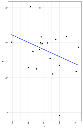

![](14-interactions_files/figure-html/unnamed-chunk-1-1.png)

]
.pull-right[
### Multivariate regression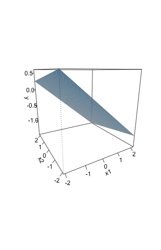

![](14-interactions_files/figure-html/unnamed-chunk-2-1.png)

]
---

### Multivariate regression with an interaction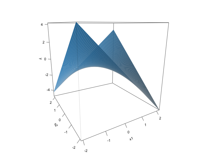

![](14-interactions_files/figure-html/unnamed-chunk-3-1.png)

---

### Example

We shall return to the data we used in the multiple regression model with two continuous variables. Here we have an outcome (Stress) that we are interested in predicting from trait Anxiety and levels of social Support.

```r
library(here)
stress.data = read.csv(here("data/stress.csv"))
library(psych)
describe(stress.data)
```

```
##         vars   n   mean     sd median trimmed    mad  min    max  range  skew
## id         1 118 488.65 295.95 462.50  485.76 372.13 2.00 986.00 984.00  0.10
## Anxiety    2 118   7.61   2.49   7.75    7.67   2.26 0.70  14.64  13.94 -0.18
## Stress     3 118   5.18   1.88   5.27    5.17   1.65 0.62  10.32   9.71  0.08
## Support    4 118   8.73   3.28   8.52    8.66   3.16 0.02  17.34  17.32  0.18
## group*     5 118   1.53   0.50   2.00    1.53   0.00 1.00   2.00   1.00 -0.10
##         kurtosis    se
## id         -1.29 27.24
## Anxiety     0.28  0.23
## Stress      0.22  0.17
## Support     0.19  0.30
## group*     -2.01  0.05
```

---

```r
i.model1 = lm(Stress ~ Anxiety + Support + Anxiety:Support, 
              data = stress.data)
i.model2 = lm(Stress ~ Anxiety*Support, data = stress.data)
```

Both methods of specifying the interaction above will work in R. Using the `*` tells R to create both the (partial) main effects and interaction effect. Note, however that the following code *gives you the wrong results*:

```r
imodel_bad = lm(Stress ~ Anxiety:Support, 
                data = stress.data) # this does not create main effects. 
#It is VERY WRONG
```

---

```r
i.model1 = lm(Stress ~ Anxiety*Support, data = stress.data)
summary(i.model1)
```

```
## 
## Call:
## lm(formula = Stress ~ Anxiety * Support, data = stress.data)
## 
## Residuals:
##     Min      1Q  Median      3Q     Max 
## -3.8163 -1.0783  0.0373  0.9200  3.6109 
## 
## Coefficients:
##                 Estimate Std. Error t value Pr(>|t|)    
## (Intercept)     -2.73966    1.12101  -2.444  0.01606 *  
## Anxiety          0.61561    0.13010   4.732 6.44e-06 ***
## Support          0.66697    0.09547   6.986 2.02e-10 ***
## Anxiety:Support -0.04174    0.01309  -3.188  0.00185 ** 
## ---
## Signif. codes:  0 '***' 0.001 '**' 0.01 '*' 0.05 '.' 0.1 ' ' 1
## 
## Residual standard error: 1.462 on 114 degrees of freedom
## Multiple R-squared:  0.4084,	Adjusted R-squared:  0.3928 
## F-statistic: 26.23 on 3 and 114 DF,  p-value: 5.645e-13
```
---

### Conceptual interpretation

`$$\hat{Y} = b_{0} + b_{1}X + b_{2}Z + b_{3}XZ$$`

You can interpret the interaction term in the same way you normally interpret a slope coefficient -- this is the effect of the interaction controlling for other variables in the model.

You can also interpret the intercept the same way as before (the expected value of Y when all predictors are 0).

But here, `$b_1$` is the effect of X on Y when Z is equal to 0.

---

### Conceptual interpretation
`$$\hat{Y} = b_{0} + b_{1}X + b_{2}Z + b_{3}XZ$$`

**Lower-order terms** change depending on the values of the higher-order terms. The value of `$b_1$` and `$b_2$` will change depending on the value of `$b_3$`. 
- These values represent "conditional effects" (because the value is conditional on the level of the other variable). In many cases, the value and significance test with these terms is either meaningless (if Z is never equal to 0) or unhelpful, as these values and significance change across the data.

**Higher-order terms** are those terms that represent interactions. `$b_3$` is a higher-order term. 
- This value represents how much the slope of X changes for every 1-unit increase in Z AND how much the slope of Z changes for everyone 1-unit increase in X.

???

Is `$b_0$` a higher-order or lower-order term?

Ask what values `$b_0$` depends on -- both intercept and slope. Maybe be helpful to use paper to represent plane.

---
### Conceptual interpretation

Higher-order interaction terms represent:
- the change in the slope of X as a function of Z
- the degree of curvature in the regression plane
- the linear effect of the product of independent variables

```r
stress.data$AxS = stress.data$Anxiety*stress.data$Support
head(stress.data[,c("Anxiety", "Support", "AxS")])
```

```
##    Anxiety Support       AxS
## 1 10.18520  6.1602  62.74287
## 2  5.58873  8.9069  49.77826
## 3  6.58500 10.5433  69.42763
## 4  8.95430 11.4605 102.62076
## 5  7.59910  5.5516  42.18716
## 6  8.15600  7.5117  61.26543
```

---

```r
summary(lm(Stress ~ Anxiety + Support + AxS, data = stress.data))
```

```
## 
## Call:
## lm(formula = Stress ~ Anxiety + Support + AxS, data = stress.data)
## 
## Residuals:
##     Min      1Q  Median      3Q     Max 
## -3.8163 -1.0783  0.0373  0.9200  3.6109 
## 
## Coefficients:
##             Estimate Std. Error t value Pr(>|t|)    
## (Intercept) -2.73966    1.12101  -2.444  0.01606 *  
## Anxiety      0.61561    0.13010   4.732 6.44e-06 ***
## Support      0.66697    0.09547   6.986 2.02e-10 ***
## AxS         -0.04174    0.01309  -3.188  0.00185 ** 
## ---
## Signif. codes:  0 '***' 0.001 '**' 0.01 '*' 0.05 '.' 0.1 ' ' 1
## 
## Residual standard error: 1.462 on 114 degrees of freedom
## Multiple R-squared:  0.4084,	Adjusted R-squared:  0.3928 
## F-statistic: 26.23 on 3 and 114 DF,  p-value: 5.645e-13
```

---

```r
summary(lm(Stress ~ Anxiety*Support, data = stress.data))
```

They're the same!!
---

## Conditional effects and simple slopes

The regression line estimated in this model is quite difficult to interpret on its own. A good strategy is to decompose the regression equation into **simple slopes**, which are determined by calculating the conditional effects at a specific level of the moderating variable.

- Simple slope: the equation for Y on X at differnt levels of Z; but also refers to only the coefficient for X in this equation

- Conditional effect: the slope coefficients in the full regression model which can change. These are the lower-order terms associated with a variable. E.g., X has a conditional effect on Y.

Which variable is the "predictor" (X) and which is the "moderator" (Z)?

---

The conditional nature of these effects is easiest to see by "plugging in" different values for one of your variables. Return to the regression equation estimated in our stress data:

`$$\hat{Stress} = -2.74 + 0.62(\text{Anx})+ 0.67(\text{Sup})+ -0.04(\text{Anx} \times \text{Sup})$$`
--
**Set Support to 5**
$$
`\begin{aligned}
\hat{Stress} &= -2.74 + 0.62(\text{Anx})+ 0.67(5)+ -0.04(\text{Anx} \times 5) \\
&= -2.74 + 0.62(\text{Anx})+ 3.35+ -0.2(\text{Anx}) \\
&= 0.61 + 0.42(\text{Anx})
\end{aligned}`
$$
--
**Set Support to 10**
$$
`\begin{aligned}
\hat{Stress} &= -2.74 + 0.62(\text{Anx})+ 0.67(10)+ -0.04(\text{Anx} \times 10) \\
&= -2.74 + 0.62(\text{Anx})+ 6.7+ -0.4(\text{Anx}) \\
&= 3.96 + 0.22(\text{Anx})
\end{aligned}`
$$

---

## Interaction shapes

Often we graph the simple slopes as a way to understand the interaction. Interpreting the shape of an interaction can be done using the numbers alone, but it requires a lot of calculation and mental rotation. For those reasons, consider it a requirement that you graph interactions in order to interpret them.

---
## Interaction shapes
### Ordinal interactions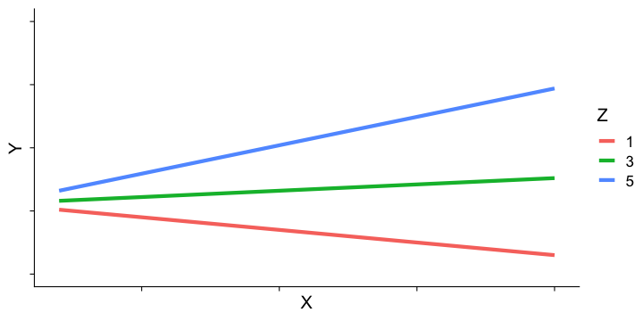

![](14-interactions_files/figure-html/unnamed-chunk-12-1.png)

---
## Interaction shapes
### Cross-over (disordinal) interactions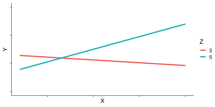

![](14-interactions_files/figure-html/unnamed-chunk-13-1.png)

---

```r
library(sjPlot)
plot_model(imodel, type = "int")
```

![](14-interactions_files/figure-html/unnamed-chunk-14-1.png)

---

```r
plot_model(imodel, type = "int", mdrt.values = "meansd")
```

![](14-interactions_files/figure-html/unnamed-chunk-15-1.png)

---

```r
plot_model(imodel, type = "pred", terms = c("Support", "Anxiety"), mdrt.values = "meansd")
```

![](14-interactions_files/figure-html/unnamed-chunk-16-1.png)

---

### Simple slopes - Significance tests

Recall that the slope at any particular value is a combination of both `$b_1$` and `$b_3$` 
`$$\large \hat{Y} = (b_{0} + b_{2}Z) + (b_{1} + b_{3}Z)X$$`
`$$\large se_{b@z} = \sqrt{se_{b_1}^2 + (2 * Z * cov_{b_1b_3})+ (Z^2 se_{b_3}^2)}$$`
In this formula, `$cov_{b_1b_3}$` refers to the covariance of the coefficients, not the covariance of the variables. This may seem a strange concept, as we only ever have one value for `$b_1$` and `$b_3$` -- the covariance of these coefficients refer to idea that if we randomly sample from a population, estimate the coefficients each time, and then examine the covariance of coefficients across random samples, it will not be 0.

---
### Simple slopes - Significance tests

```r
round(vcov(imodel),4)
```

```
##                 (Intercept) Anxiety Support Anxiety:Support
## (Intercept)          1.2567 -0.1330 -0.0966          0.0100
## Anxiety             -0.1330  0.0169  0.0110         -0.0015
## Support             -0.0966  0.0110  0.0091         -0.0011
## Anxiety:Support      0.0100 -0.0015 -0.0011          0.0002
```

We can use the standard error of the slope to estimate whether or not it is significanly different from 0.

.pull-left[
`$$\large \hat{Y} = (b_{0} + b_{2}Z) + (b_{1} + b_{3}Z)X$$`
`$$\large t = \frac{(b_{1} + b_{3}Z)}{se_{b@z}}$$`
`$$df = N-p-1$$`
]

---

#### Example

`$$\hat{Stress} = -2.74 + 0.62(\text{Anx})+ 0.67(\text{Sup})+ -0.04(\text{Anx} \times \text{Sup})$$`

We want to know whether anxiety is a significant predictor of stress at different levels of support.

```r
library(reghelper)
simple_slopes(imodel, levels = list(Support = c(4,6,8,10,12)))
```

```
##   Anxiety Support Test Estimate Std. Error t value  df  Pr(>|t|) Sig.
## 1  sstest       4        0.4486     0.0886  5.0617 114 1.610e-06  ***
## 2  sstest       6        0.3652     0.0733  4.9791 114 2.289e-06  ***
## 3  sstest       8        0.2817     0.0654  4.3095 114 3.488e-05  ***
## 4  sstest      10        0.1982     0.0674  2.9424 114  0.003946   **
## 5  sstest      12        0.1147     0.0786  1.4600 114  0.147036
```

If you don't list levels, then this function will test simple slopes at the mean and 1 SD above and below the mean. 
---
## Simple slopes - Significance tests

What if you want to compare slopes to each other? How would we test this?

The test of the interaction coefficient is equivalent to the test of the difference in slopes at levels of Z separated by 1 unit.

```r
coef(summary(imodel))
```

```
##                    Estimate Std. Error   t value     Pr(>|t|)
## (Intercept)     -2.73966246 1.12100519 -2.443934 1.606052e-02
## Anxiety          0.61561220 0.13010161  4.731780 6.435373e-06
## Support          0.66696689 0.09547464  6.985802 2.017698e-10
*## Anxiety:Support -0.04174076 0.01309328 -3.187954 1.849736e-03
```

---

## Centering

The regression equation built using the raw data is not only diffiuclt to interpret, but often the terms displayed are not relevant to the hypotheses we're interested. 
- `$b_0$` is the expected value when all predictors are 0, but this may never happen in real life
- `$b_1$` is the slope of X when Z is equal to 0, but this may not ever happen either.

**Centering** your variables by subracting the mean from all values can improve the interpretation of your results. 
- Remember, a linear transformation does not change associations (correlations) between variables. In this case, it only changes the interpretation for some coefficients
---

```r
stress.data = stress.data %>%
  mutate(Anxiety.c = Anxiety - mean(Anxiety),
         Support.c = Support - mean(Support))
head(stress.data[,c("Anxiety", "Anxiety.c", "Support", "Support.c")])
```

```
##    Anxiety   Anxiety.c Support  Support.c
## 1 10.18520  2.57086873  6.1602 -2.5697997
## 2  5.58873 -2.02560127  8.9069  0.1769003
## 3  6.58500 -1.02933127 10.5433  1.8133003
## 4  8.95430  1.33996873 11.4605  2.7305003
## 5  7.59910 -0.01523127  5.5516 -3.1783997
## 6  8.15600  0.54166873  7.5117 -1.2182997
```

Why did we not center Y (Stress)?

---

```r
summary(lm(Stress ~ Anxiety.c*Support.c, data = stress.data))
```

```
## 
## Call:
## lm(formula = Stress ~ Anxiety.c * Support.c, data = stress.data)
## 
## Residuals:
##     Min      1Q  Median      3Q     Max 
## -3.8163 -1.0783  0.0373  0.9200  3.6109 
## 
## Coefficients:
##                     Estimate Std. Error t value Pr(>|t|)    
## (Intercept)          4.99580    0.14647  34.108  < 2e-16 ***
## Anxiety.c            0.25122    0.06489   3.872 0.000181 ***
## Support.c            0.34914    0.05238   6.666 9.82e-10 ***
## Anxiety.c:Support.c -0.04174    0.01309  -3.188 0.001850 ** 
## ---
## Signif. codes:  0 '***' 0.001 '**' 0.01 '*' 0.05 '.' 0.1 ' ' 1
## 
## Residual standard error: 1.462 on 114 degrees of freedom
## Multiple R-squared:  0.4084,	Adjusted R-squared:  0.3928 
## F-statistic: 26.23 on 3 and 114 DF,  p-value: 5.645e-13
```

---

```r
summary(imodel)
```

---
 
## Standardized regression equation

So far, we've only discussed the unstandardized regression equation. If you're interested in getting the standardized regression equation, you can follow the same procedure of standardizing your variables first and then entering them into your linear model.

An important note: You must take the product of the Z-scores, not the Z-score of the products to get the correct regression model.

.pull-left[
#### This is OK

```r
Y ~ z(X) + z(Z) + z(X)*z(Z)

Y ~ z(X)*z(Z) 
```

]

.pull-right[
#### This is not OK

```r
Y ~ z(X) + z(Z) + z(X*Z) 
```

]

---

```r
stress.data = stress.data %>%
  mutate(zStress = scale(Stress), 
         zAnxiety = scale(Anxiety), 
         zSupport = scale(Support))
head(stress.data[,c("zStress", "zAnxiety", "zSupport")])
```

```
##       zStress     zAnxiety    zSupport
## 1 -1.05630148  1.033649700 -0.78410538
## 2  0.97450140 -0.814418147  0.05397639
## 3  0.52978175 -0.413855421  0.55327992
## 4  1.87547440  0.538751068  0.83313888
## 5  0.04640497 -0.006123922 -0.96980334
## 6 -0.02939564  0.217784639 -0.37173144
```
---

```r
zmodel = lm(zStress ~ zAnxiety*zSupport, stress.data)
summary(zmodel)
```

```
## 
## Call:
## lm(formula = zStress ~ zAnxiety * zSupport, data = stress.data)
## 
## Residuals:
##      Min       1Q   Median       3Q      Max 
## -2.03400 -0.57471  0.01989  0.49037  1.92453 
## 
## Coefficients:
##                   Estimate Std. Error t value Pr(>|t|)    
## (Intercept)       -0.09818    0.07807  -1.258 0.211093    
## zAnxiety           0.33302    0.08602   3.872 0.000181 ***
## zSupport           0.60987    0.09149   6.666 9.82e-10 ***
## zAnxiety:zSupport -0.18134    0.05688  -3.188 0.001850 ** 
## ---
## Signif. codes:  0 '***' 0.001 '**' 0.01 '*' 0.05 '.' 0.1 ' ' 1
## 
## Residual standard error: 0.7792 on 114 degrees of freedom
## Multiple R-squared:  0.4084,	Adjusted R-squared:  0.3928 
## F-statistic: 26.23 on 3 and 114 DF,  p-value: 5.645e-13
```

---

```r
zmodel = lm(zStress ~ zAnxiety + zSupport + zAxS, stress.data)
summary(zmodel)
```

```
## 
## Call:
## lm(formula = zStress ~ zAnxiety + zSupport + zAxS, data = stress.data)
## 
## Residuals:
##      Min       1Q   Median       3Q      Max 
## -2.03400 -0.57471  0.01989  0.49037  1.92453 
## 
## Coefficients:
##               Estimate Std. Error t value Pr(>|t|)    
## (Intercept)  2.833e-17  7.173e-02   0.000  1.00000    
## zAnxiety     8.161e-01  1.725e-01   4.732 6.44e-06 ***
## zSupport     1.165e+00  1.668e-01   6.986 2.02e-10 ***
## zAxS        -5.003e-01  1.569e-01  -3.188  0.00185 ** 
## ---
## Signif. codes:  0 '***' 0.001 '**' 0.01 '*' 0.05 '.' 0.1 ' ' 1
## 
## Residual standard error: 0.7792 on 114 degrees of freedom
## Multiple R-squared:  0.4084,	Adjusted R-squared:  0.3928 
## F-statistic: 26.23 on 3 and 114 DF,  p-value: 5.645e-13
```

---
class: inverse

## Next time...

Mixing categorical and continuous predictors

Factorial ANOVA