class: center, middle, inverse, title-slide # Univariate regression --- ## Last time - Correlation as inferential test - Power - Fisher's r to z transformation - Correlation matrices - Interpreting effect size --- ## Today **Regression** - What is it? Why is it useful - Nuts and bolts - Equation - Ordinary least squares - Interpretation --- ## Regression Regression is a general data analytic system, meaning lots of things fall under the umbrella of regression. This system can handle a variety of forms of relations, although all forms have to be specified in a linear way. Usefully, we can incorporate IVs of all nature -- continuous, categorical, nominal, ordinal.... The output of regression includes both effect sizes and, if using frequentist or Bayesian software, statistical significance. We can also incorporate multiple influences (IVs) and account for their intercorrelations. --- ### Regression - **Scientific** use: explaining the influence of one or more variables on some outcome. + Does this intervention affect reaction time? + Does self-esteem predict relationship quality? - **Prediction** use: We can develop models based on what's happened in the past to predict what will happen in the figure. + Insurance premiums + Graduate school... success? - **Adjustment**: Statistically control for known effects + If everyone had the same level of SES, would abuse still be associated with criminal behavior? --- ## Regression equation What is a regression equation? - Functional relationship - Ideally like a physical law `\((E = MC^2)\)` - In practice, it's never as robust as that How do we uncover the relationship? --- ### How does Y vary with X? - The regression of Y (DV) on X (IV) corresponds to the line that gives the mean value of Y corresponding to each possible value of X - `\(\large E(Y|X)\)` - "Our best guess" regardless of whether our model includes categories or continuous predictor variables --- ## Regression Equation `$$\Large Y = b_{0} + b_{1}X +e$$` `$$\Large \hat{Y} = b_{0} + b_{1}X$$` ??? `\(\hat{Y}\)` signifies the predicted score -- no error The difference between the predicted and observed score is the residual ($e_i$) There is a different e value for each observation in the dataset --- ## OLS - How do we find the regression estimates? - Ordinary Least Squares (OLS) estimation - Minimizes deviations $$ min\sum(Y_{i}-\hat{Y})^{2} $$ - Other estimation procedures possible (and necessary in some cases) --- <!-- --> --- <!-- --> --- <!-- --> --- <!-- --> --- <!-- --> ## compare to bad fit --- `$$\Large Y = b_{0} + b_{1}X +e$$` `$$\Large \hat{Y} = b_{0} + b_{1}X$$` `$$\Large Y_i = \hat{Y_i} + e_i$$` `$$\Large e_i = Y_i - \hat{Y_i}$$` --- ## OLS The line that yields the smallest sum of squared deviations `$$\Large \Sigma(Y_i - \hat{Y_i})^2$$` `$$\Large = \Sigma(Y_i - (b_0+b_{1}X_i))^2$$` `$$\Large = \Sigma(e_i)^2$$` -- In order to find the OLS solution, you could try many different coefficients `\((b_0 \text{ and } b_{1})\)` until you find the one with the smallest sum squared deviation. Luckily, there are simple calculations that will yield the OLS solution every time. --- ## Regression coefficient, `\(b_{1}\)` `$$\large b_{1} = \frac{cov_{XY}}{s_{x}^{2}} = r_{xy} \frac{s_{y}}{s_{x}}$$` `$$\large r_{xy} = \frac{s_{xy}}{s_xs_y}$$` - The regression coefficient (slope) equals the estimated change in Y for a 1-unit change in X --- `$$\large b_{1} = r_{xy} \frac{s_{y}}{s_{x}}$$` If the variance of both X and Y is equal to 1: `$$\large b_1 = \frac{s_{xy}}{s_xs_y} = \frac{s_{xy}}{s_x^2}=\frac{r_{xy}}{1^2} = \beta_{yx} = b_{yx}^*$$` --- ## Standardized regression equation `$$\large Y = b_{yx}^*X+e$$` `$$\large b_{yx}^* = b_{yx}\frac{s_x}{s_y}$$` -- According to this regression equation, when `\(X = 0, Y = 0\)`. Our interpretation of the coefficient is that a one-standard deviation increase in X is associated with a `\(b_{yx}^*\)` standard deviation increase in Y. Our regression coefficient is equivalent to the correlation coefficient *when we have only one predictor in our model.* --- ## Estimating the intercept, `\(b_0\)` - intercept serves to adjust for differences in means between X and Y `$$\Large \hat{Y} = \bar{Y} + r_{xy} \frac{s_{y}}{s_{x}}(X-\bar{X})$$` - if standardized, intercept drops out - otherwise, intercept is where regression line crosses the y-axis at X = 0 ??? ##Make this point - Also, notice that when `\(X = \bar{X}\)` the regression line goes through `\(\bar{Y}\)` ??? `$$\Large b_0 = \bar{Y} - b_1\bar{X}$$` --- ## Example ```r galton.data <- psychTools::galton head(galton.data) ``` ``` ## parent child ## 1 70.5 61.7 ## 2 68.5 61.7 ## 3 65.5 61.7 ## 4 64.5 61.7 ## 5 64.0 61.7 ## 6 67.5 62.2 ``` ```r describe(galton.data, fast = T) ``` ``` ## vars n mean sd min max range se ## parent 1 928 68.31 1.79 64.0 73.0 9 0.06 ## child 2 928 68.09 2.52 61.7 73.7 12 0.08 ``` ```r cor(galton.data) ``` ``` ## parent child ## parent 1.0000000 0.4587624 ## child 0.4587624 1.0000000 ``` --- If we regress child height onto parents': ```r r = cor(galton.data)[2,1] m_parent = mean(galton.data$parent) m_child = mean(galton.data$child) s_parent = sd(galton.data$parent) s_child = sd(galton.data$child) (b1 = r*(s_child/s_parent)) ``` ``` ## [1] 0.6462906 ``` ```r (b0 = m_child - b1*m_parent) ``` ``` ## [1] 23.94153 ``` How will this change if we regress parent height onto child height? --- ```r (b1 = r*(s_child/s_parent)) ``` ``` ## [1] 0.6462906 ``` ```r (b0 = m_child - b1*m_parent) ``` ``` ## [1] 23.94153 ``` ```r (b1 = r*(s_parent/s_child)) ``` ``` ## [1] 0.3256475 ``` ```r (b0 = m_parent - b1*m_child) ``` ``` ## [1] 46.13535 ``` --- ## In `R` ```r fit.1 <- lm(child ~ parent, data = galton.data) summary(fit.1) ``` ``` ## ## Call: ## lm(formula = child ~ parent, data = galton.data) ## ## Residuals: ## Min 1Q Median 3Q Max ## -7.8050 -1.3661 0.0487 1.6339 5.9264 ## ## Coefficients: ## Estimate Std. Error t value Pr(>|t|) ## (Intercept) 23.94153 2.81088 8.517 <2e-16 *** ## parent 0.64629 0.04114 15.711 <2e-16 *** ## --- ## Signif. codes: 0 '***' 0.001 '**' 0.01 '*' 0.05 '.' 0.1 ' ' 1 ## ## Residual standard error: 2.239 on 926 degrees of freedom ## Multiple R-squared: 0.2105, Adjusted R-squared: 0.2096 ## F-statistic: 246.8 on 1 and 926 DF, p-value: < 2.2e-16 ``` ??? **Things to discuss** - Coefficient estimates - Statistical tests (covered in more detail soon) --- <!-- --> --- ### Data, predicted, and residuals ```r library(broom) model_info = augment(fit.1) head(model_info) ``` ``` ## # A tibble: 6 x 9 ## child parent .fitted .se.fit .resid .hat .sigma .cooksd .std.resid ## <dbl> <dbl> <dbl> <dbl> <dbl> <dbl> <dbl> <dbl> <dbl> ## 1 61.7 70.5 69.5 0.116 -7.81 0.00270 2.22 0.0165 -3.49 ## 2 61.7 68.5 68.2 0.0739 -6.51 0.00109 2.23 0.00462 -2.91 ## 3 61.7 65.5 66.3 0.137 -4.57 0.00374 2.23 0.00787 -2.05 ## 4 61.7 64.5 65.6 0.173 -3.93 0.00597 2.24 0.00931 -1.76 ## 5 61.7 64 65.3 0.192 -3.60 0.00735 2.24 0.00966 -1.62 ## 6 62.2 67.5 67.6 0.0807 -5.37 0.00130 2.23 0.00374 -2.40 ``` ```r describe(model_info) ``` ``` ## vars n mean sd median trimmed mad min max range skew ## child 1 928 68.09 2.52 68.20 68.12 2.97 61.70 73.70 12.00 -0.09 ## parent 2 928 68.31 1.79 68.50 68.32 1.48 64.00 73.00 9.00 -0.04 ## .fitted 3 928 68.09 1.16 68.21 68.10 0.96 65.30 71.12 5.82 -0.04 ## .se.fit 4 928 0.10 0.03 0.09 0.09 0.02 0.07 0.21 0.13 1.53 ## .resid 5 928 0.00 2.24 0.05 0.06 2.26 -7.81 5.93 13.73 -0.24 ## .hat 6 928 0.00 0.00 0.00 0.00 0.00 0.00 0.01 0.01 1.99 ## .sigma 7 928 2.24 0.00 2.24 2.24 0.00 2.22 2.24 0.01 -2.39 ## .cooksd 8 928 0.00 0.00 0.00 0.00 0.00 0.00 0.02 0.02 3.44 ## .std.resid 9 928 0.00 1.00 0.02 0.03 1.01 -3.49 2.65 6.14 -0.24 ## kurtosis se ## child -0.35 0.08 ## parent 0.05 0.06 ## .fitted 0.05 0.04 ## .se.fit 1.50 0.00 ## .resid -0.23 0.07 ## .hat 3.47 0.00 ## .sigma 8.62 0.00 ## .cooksd 17.34 0.00 ## .std.resid -0.23 0.03 ``` ??? Point out the average of the residuals is 0, just like average deviation from the mean is 0. --- ```r model_info %>% ggplot(aes(x = parent, y = .fitted)) + geom_point() + geom_smooth(se = F, method = "lm") + ggtitle(expression(paste("X is related to ", hat(Y))))+ scale_x_continuous("X") + scale_y_continuous(expression(hat(Y))) + theme_bw(base_size = 30) ``` <!-- --> --- ```r model_info %>% ggplot(aes(x = parent, y = .resid)) + geom_point() + geom_smooth(se = F, method = "lm") + ggtitle("X is always unrelated to e")+ scale_x_continuous("X") + scale_y_continuous("e") + theme_bw(base_size = 30) ``` <!-- --> --- ```r model_info %>% ggplot(aes(x = child, y = .fitted)) + geom_point() + geom_smooth(se = F, method = "lm") + ggtitle(expression(paste("Y can be related to ", hat(Y))))+ scale_x_continuous("Y") + scale_y_continuous(expression(hat(Y))) + theme_bw(base_size = 30) ``` 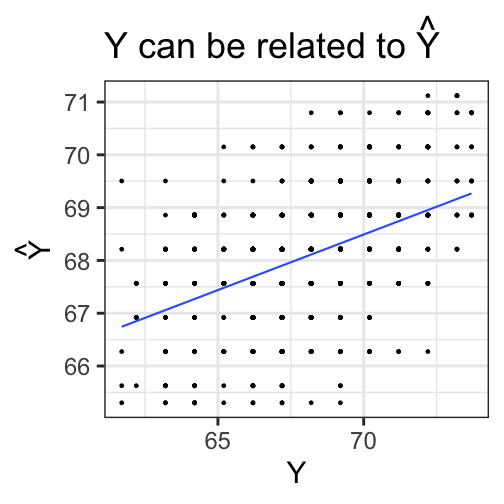<!-- --> --- ```r model_info %>% ggplot(aes(x = child, y = .resid)) + geom_point() + geom_smooth(se = F, method = "lm") + ggtitle("Y is sometimes related to e")+ scale_x_continuous("Y") + scale_y_continuous("e") + theme_bw(base_size = 25) ``` 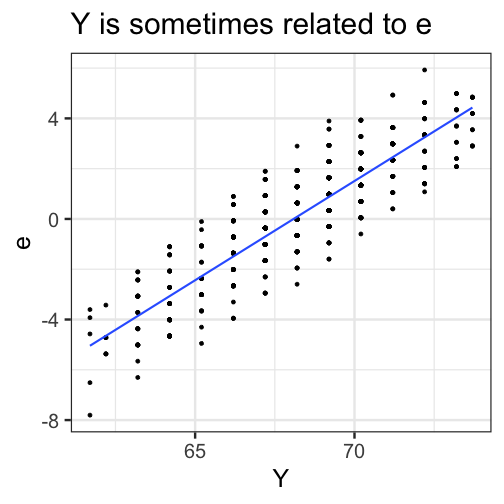<!-- --> --- ```r model_info %>% ggplot(aes(x = .fitted, y = .resid)) + geom_point() + geom_smooth(se = F, method = "lm") + ggtitle(expression(paste(hat(Y), " is always unrelated to e")))+ scale_y_continuous("e") + scale_x_continuous(expression(hat(Y))) + theme_bw(base_size = 30) ``` 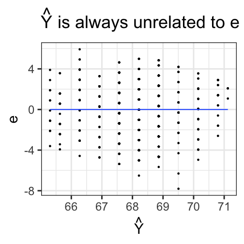<!-- --> --- ```r model_info %>% rename(y = child, x = parent) %>% select(x,y,.fitted,.resid) %>% gather("key", "value") %>% ggplot(aes(value, fill = key)) + geom_histogram(bins = 25) + guides(fill = F)+ facet_wrap(~key, scales = "free") + theme_bw(base_size = 20) ``` 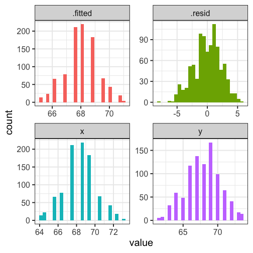<!-- --> --- class: inverse ## Next time... Statistical inferences with regression