class: center, middle, inverse, title-slide # Partial correlations --- ## Homework Homework assignment #1 has been posted! Due Friday, February 7 at 9 am. --- ## Today - path diagrams - partial and semi-partial correlations --- ## Causal relationships Does parent socioeconomic status *cause* better grades? * `\(r_{GPA,SES} = .33, b = .41\)` -- Potential confound: Peer relationships - `\(r_{SES, peer} = .29\)` - `\(r_{GPA, peer} = .37\)` ??? Don't know how variables are related, only know that they are in a perfect world, we would want to **hold constant** peer relationships - control for - partial out --- ### Does parent SES cause better grades? 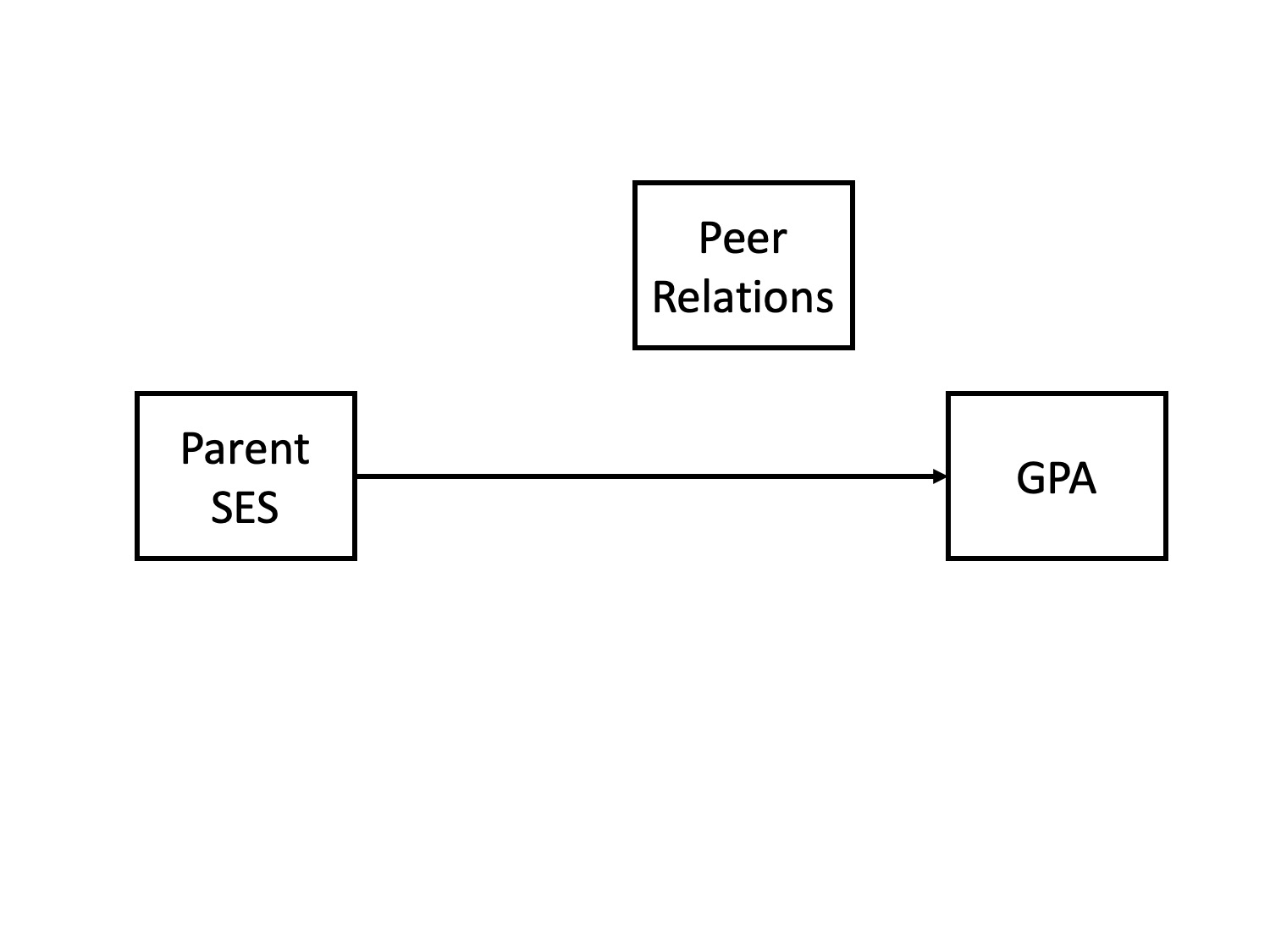 --- ### spurious relationship 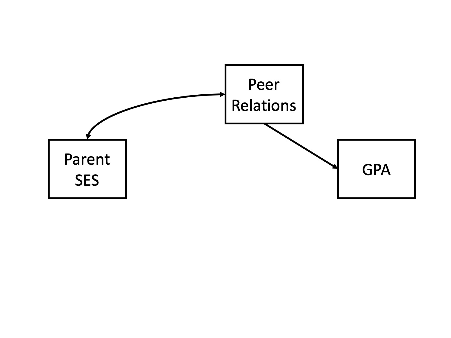 --- ### indirect (mediation) 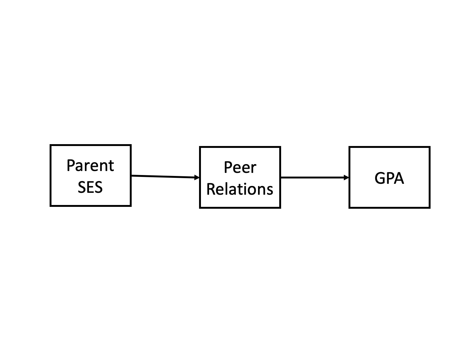 --- ### interaction (moderation) 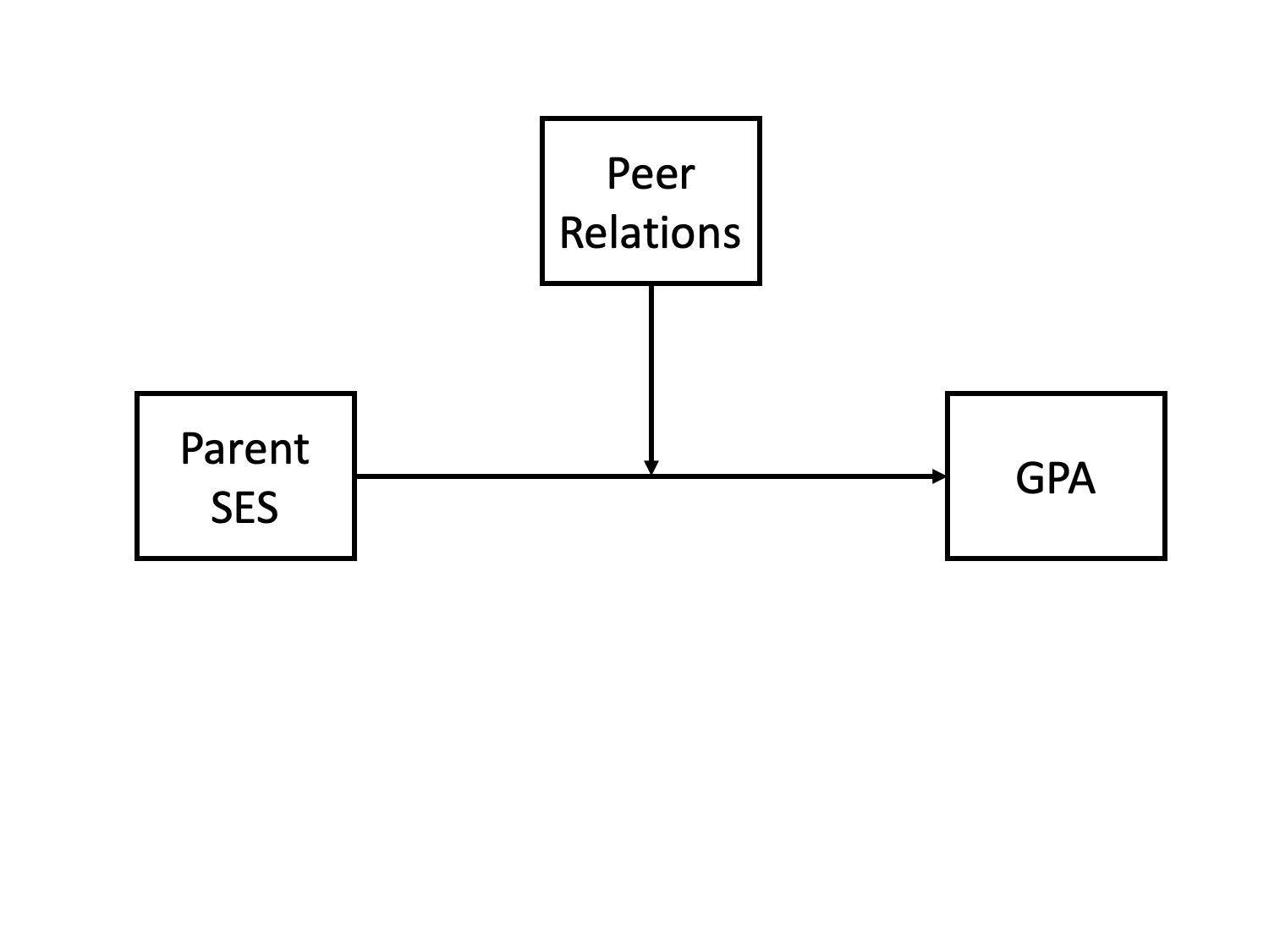 --- ### multiple causes  --- ### direct and indirect effects 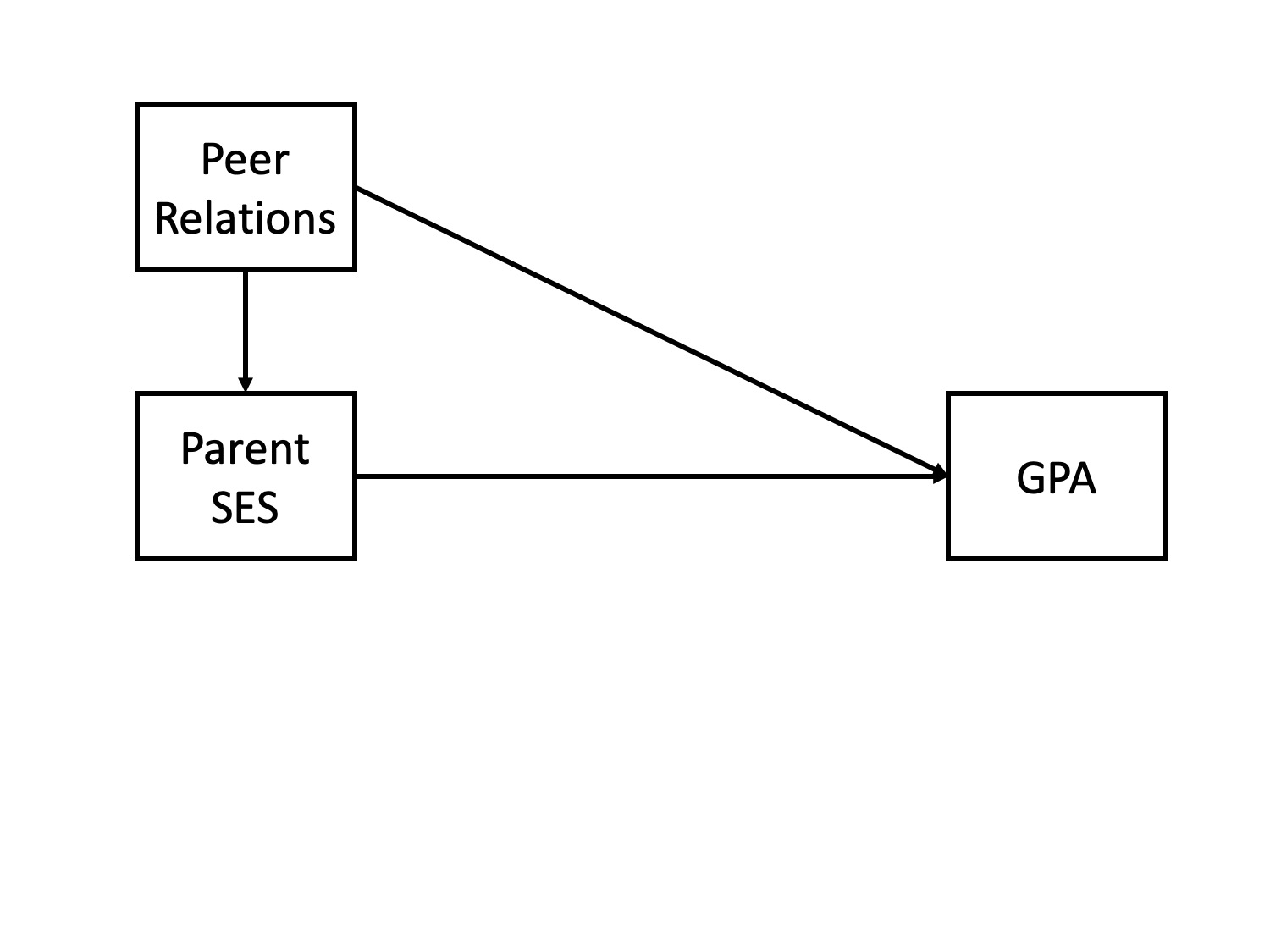 --- ### multiple regression 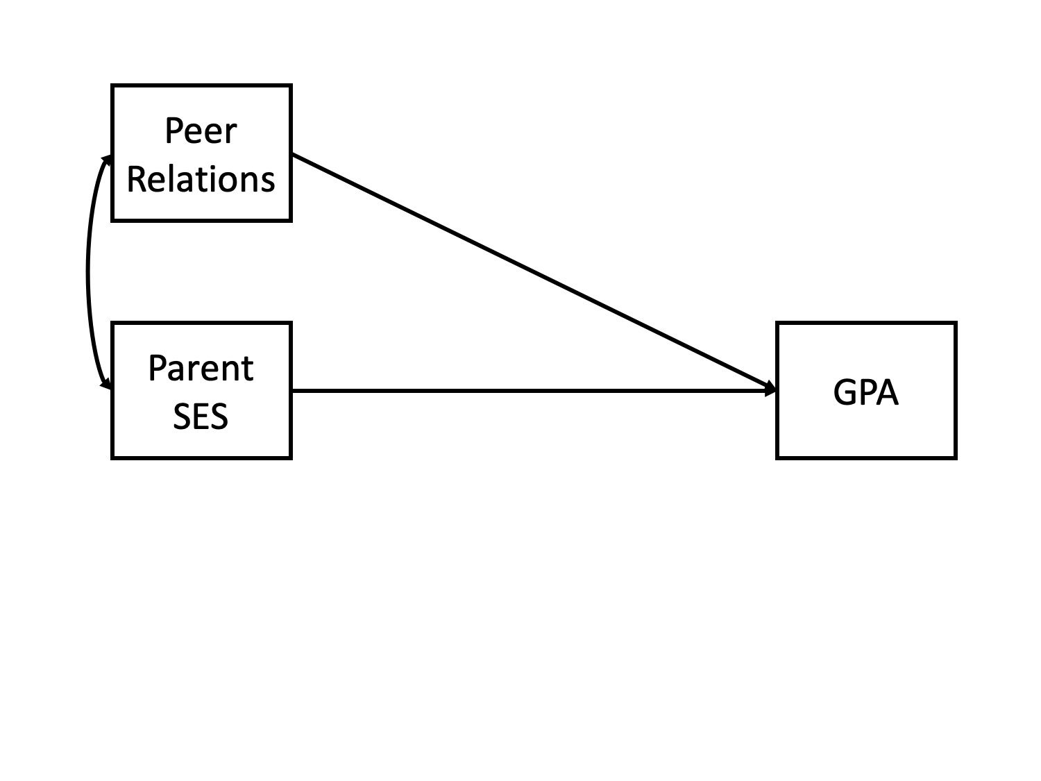 --- ## General regression model `$$\large \hat{Y} = b_0 + b_1X_1 + b_2X_2 + \dots+b_kX_k$$` This is ultimately where we want to go. Unfortunately, it's not as simply as multiplying the correlation between Y and each X by the ratio of their standard errors and stringing them together. Why? --- ## What is `\(R^2\)`? .pull-left[ 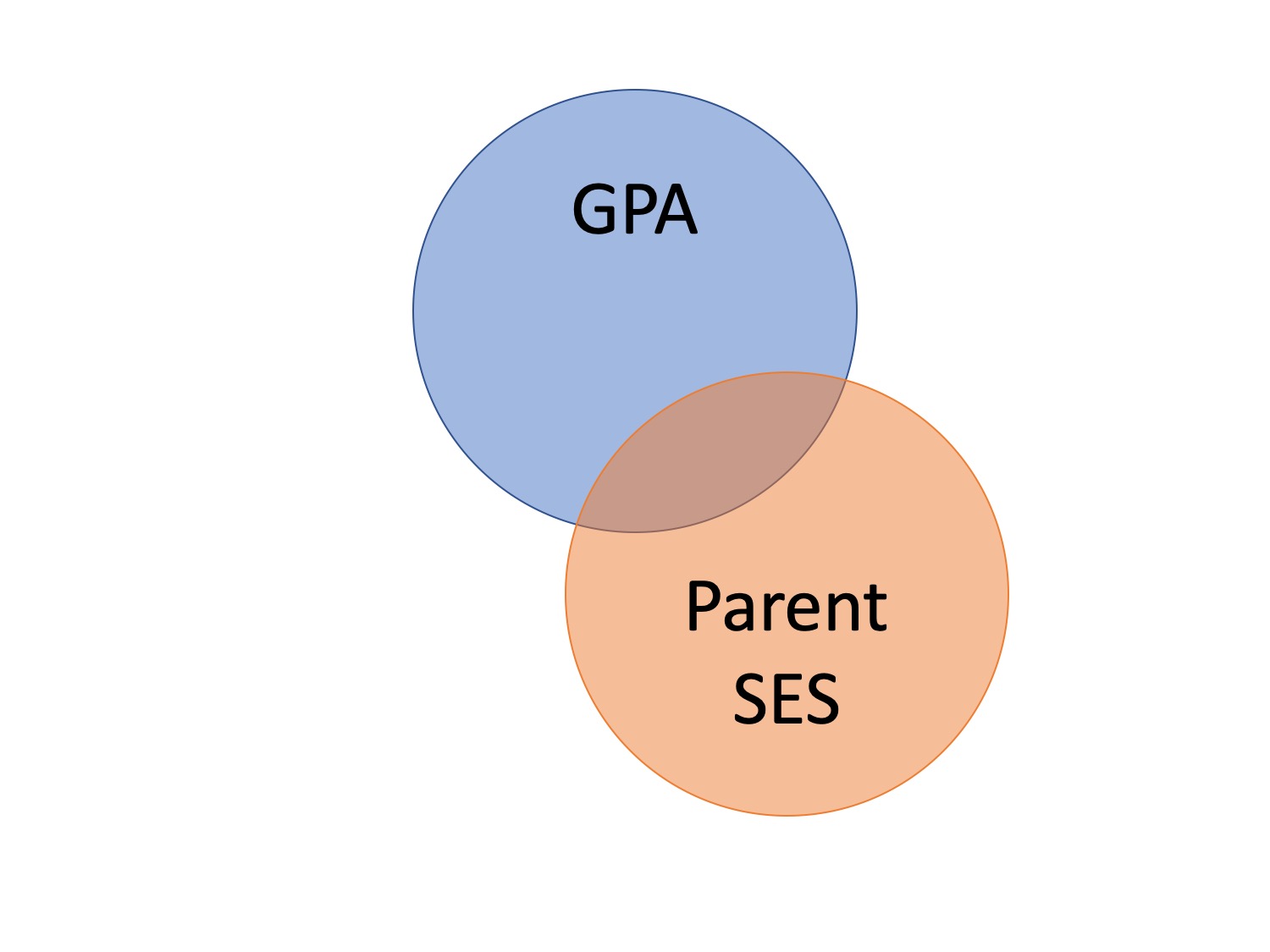 ] .pull-right[ `$$\large R^2 = \frac{s^2_{\hat{Y}}}{s^2_Y}$$` `$$\large = \frac{SS_{\text{Regression}}}{SS_Y}$$` ] --- 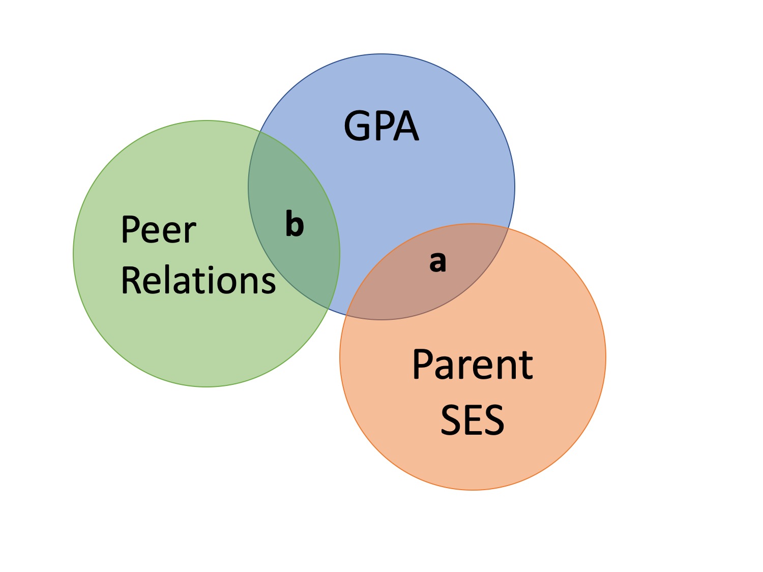 ### What is `\(R^2\)`? ---  ---  --- ### What is `\(R^2\)`?  --- ### Types of correlations Pearson product moment correlation - Zero-order correlation - Only two variables are X and Y -- Semi-partial correlation - This correlation assess the extent to which the part of `\(X_1\)` *that is independent of* of `\(X_2\)` correlates with all of Y - This is often the estimate that we refer to when we talk about **controlling for** another variable. ---  ??? the semi-partial correlation between parent SES and GPA controlling for peer relationships is a (not c), divided by all of GPA --- ### Semi-partial correlations `$$\large sr_1 = r_{Y(1.2)} = \frac{r_{Y1}-r_{Y2}r_{12}}{\sqrt{1-r^2_{12}}}$$` `$$\large sr_1^2 = R^2_{Y.12}-r^2_{Y2}$$` --- ### Types of correlations Pearson product moment correlation - Zero-order correlation - Only two variables are X and Y Semi-partial correlation - This correlation assess the extent to which the part of `\(X_1\)` *that is independent of* of `\(X_2\)` correlates with all of Y - This is often the estimate that we refer to when we talk about **controlling for** another variable. -- Partial correlation - The extent to which the part of X1 that is independent of X2 is correlated with the part of Y that is also independent of X2. ---  ---  --- ### Partial correlations `$$\large pr_1=r_{Y1.2} = \frac{r_{Y1}-r_{Y2}r_{{12}}}{\sqrt{1-r^2_{Y2}}\sqrt{1-r^2_{12}}} = \frac{r_{Y(1.2)}}{\sqrt{1-r^2_{Y_2}}}$$` --- ### What happens if X1 and X2 are uncorrelated? How does the semi-partial correlation compare to the zero-order correlation? -- `$$\large r_{Y(1.2)} = r_{Y1}$$` How does the partial correlation compare to the zero-order correlation? -- `$$\large r_{Y1.2} \neq r_{Y1}$$` --- ## When we use these? The semi-partial correlation is most often used when we want to show that some variable adds incremental variance in Y above and beyond another X variable. - e.g., predicting Alzheimer's The partial correlations most often used when some third variable, Z, is a plausible explanation of the correlation between X and Y - e.g., predicting grades --- ## Example Recall the expertise dataset, which measures a person's perception of their knowledge of personal finance (`self_perceived_knowledge`) and their performance on an objective measures of knowledge (`overclaiming_perception`). Participants also completed a test called the FINRA, which is an actual financial literacy test. ```r library(here) expertise = read.csv(here("data/expertise.csv")) ``` --- ```r round(cor(expertise[,c("self_perceived_knowledge", "overclaiming_proportion", "FINRA_score")]),2) ``` ``` ## self_perceived_knowledge overclaiming_proportion ## self_perceived_knowledge 1.00 0.48 ## overclaiming_proportion 0.48 1.00 ## FINRA_score 0.32 -0.04 ## FINRA_score ## self_perceived_knowledge 0.32 ## overclaiming_proportion -0.04 ## FINRA_score 1.00 ``` ```r library(ppcor) ``` ``` ## Loading required package: MASS ``` ```r round(spcor(expertise[,c("self_perceived_knowledge", "overclaiming_proportion", "FINRA_score")])$estimate,2) ``` ``` ## self_perceived_knowledge overclaiming_proportion ## self_perceived_knowledge 1.00 0.49 ## overclaiming_proportion 0.52 1.00 ## FINRA_score 0.38 -0.22 ## FINRA_score ## self_perceived_knowledge 0.34 ## overclaiming_proportion -0.20 ## FINRA_score 1.00 ``` --- ```r round(cor(expertise[,c("self_perceived_knowledge", "overclaiming_proportion", "FINRA_score")]),2) ``` ``` ## self_perceived_knowledge overclaiming_proportion ## self_perceived_knowledge 1.00 0.48 ## overclaiming_proportion 0.48 1.00 ## FINRA_score 0.32 -0.04 ## FINRA_score ## self_perceived_knowledge 0.32 ## overclaiming_proportion -0.04 ## FINRA_score 1.00 ``` ```r library(ppcor) round(pcor(expertise[,c("self_perceived_knowledge", "overclaiming_proportion", "FINRA_score")])$estimate,2) ``` ``` ## self_perceived_knowledge overclaiming_proportion ## self_perceived_knowledge 1.00 0.52 ## overclaiming_proportion 0.52 1.00 ## FINRA_score 0.38 -0.23 ## FINRA_score ## self_perceived_knowledge 0.38 ## overclaiming_proportion -0.23 ## FINRA_score 1.00 ``` --- ## Regression Recall that the residuals of a univariate regression equation are the part of the outcome `\((Y)\)` that is independent of the predictor `\((X)\)`. `$$\Large \hat{Y} = b_0 + b_1X$$` `$$\Large e_i = Y_i - \hat{Y_i}$$` We can use this to construct a measure of `\(X_1\)` that is independent of `\(X_2\)`: `$$\Large \hat{X}_{1.2} = b_0 + b_1X_2$$` `$$\Large e_{X_1} = X_1 - \hat{X}_{1.2}$$` --- We can either correlate that value with Y, to calculate our semi-partial correlation: `$$\Large r_{e_{X_1},Y} = r_{Y(1.2)}$$` Or we can calculate a measure of Y that is also independent of `\(X_2\)` and correlate that with our `\(X_1\)` residuals. `$$\Large \hat{Y} = b_0 + b_1X_2$$` `$$\Large e_{Y} = Y - \hat{Y}$$` `$$\Large r_{e_{X_1},e_{Y}} = r_{Y1.2}$$` --- ### Example ```r # create measure of perceived knowledge independent of FINRA score mod.know = lm(self_perceived_knowledge ~ FINRA_score, data = expertise) expertise.know = broom::augment(mod.know) # create measure of overclaiming independent of FINRA score mod.over = lm(overclaiming_proportion ~ FINRA_score, data = expertise) expertise.over = broom::augment(mod.over) #semi-parital cor(expertise.know$.resid, expertise$overclaiming_proportion) ``` ``` ## [1] 0.5201425 ``` ```r #parital cor(expertise.know$.resid, expertise.over$.resid) ``` ``` ## [1] 0.5205143 ``` --- class: inverse ## Next time... Multiple regression!!